Geometric probability
An extension of the topic of probability and the area of figures. When we draw a point uniformly from a figure, the probability of landing in a subregion does not depend on counting cases — it equals the ratio of areas: P = favorable area / total area. This extends the classical definition to cases with infinitely many outcomes — pioneered by Buffon's needle problem (around 1777).
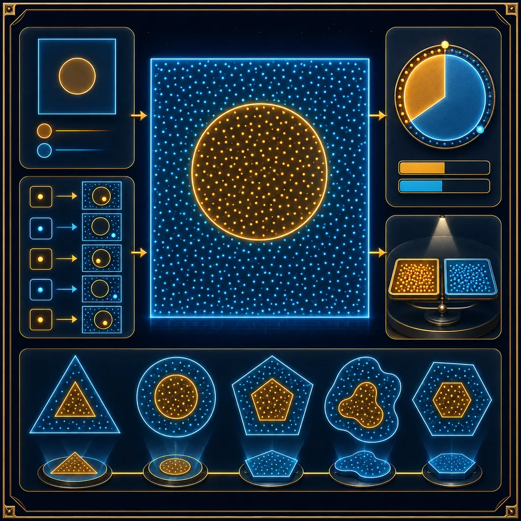
I’ll give you a target probability of landing in the circle — tune the radius r with the slider to reach it. P = πr².
What just happened?
We draw a point uniformly from a square of side 1 (area = 1), with a circle of radius inscribed in it — this is the favorable region. The probability of landing in the circle does not depend on counting cases (as with a die roll), because there are infinitely many points. We compute it as the ratio of areas — and that is exactly the share of blue points among all of them.
Geometric probability:
Here the favorable area is (circle), and the total area is (square), so . This extends the classical definition of probability to cases with infinitely many equally likely outcomes.
The invariant — why NOT always ½:
The probability changes together with the size of the favorable region — it equals the ratio of measures, not a constant ½. The key assumption is the uniformity of the sampling: every point of the figure is equally likely. Analogously we compute it for lengths on a segment () or volumes in space.
Where did this concept come from?
The first example of geometric probability was the famous Buffon’s needle problem (Georges-Louis Leclerc de Buffon, 18th century): we toss a needle onto a floor of parallel boards and ask what the chance is that the needle crosses a line between the boards. The answer leads directly to a ratio of measures (and surprisingly — to the number ). This idea also underlies Monte Carlo methods — estimating quantities through random sampling.
What does this mean in practice?
When the “event space” is continuous (a random point, a random moment in time, a random length), you cannot count cases — instead we draw regions and divide their measures. The scattered grid of points in the simulation only estimates this ratio (hits/N ≈ P), but the formula itself is exact.
Why you need this for the exam:
In geometric-probability problems the trick is always the same: draw the total region and the favorable region, compute their measures (area, length, volume) and divide one by the other. Watch out for the uniformity assumption — without it the formula does not work.
Remember: with uniform sampling, probability = measure of the favorable region / measure of the total region. Not ½ “by eye” — the exact ratio of areas.
Theory & formulas
Definition
For a point drawn uniformly from a figure, the probability of landing in a subregion is the ratio of measures:
When to use it
When there are infinitely many outcomes (a random point in a figure, a random moment in time) — the classical definition based on counting fails.
Related
Buffon's needle and Monte Carlo methods rest precisely on the measure of regions.
Notation: the whole region, the favorable region, probability.
Frequently asked questions
›What does geometric probability equal?
The ratio of measures: the favorable region's area to the total region's area (for a uniform draw).
›When is geometric probability used?
When there are infinitely many outcomes — e.g. a random point in a figure, a random moment in time.
›What is geometric probability connected with?
With Buffon's needle problem and Monte Carlo methods (estimation through random sampling).
Teaching? Embed this experiment on your site.
Free widget — paste it on your school site, blog or notes. It links to the full version.