Sorting algorithms — complexity
An extension of the topic of computational complexity and functions (beyond the curriculum — computer science). Simple bubble sort performs ~n² comparisons, while a clever one (merge sort) performs ~n·log n — for large n the difference is enormous (for n=1000 that is a hundred times fewer operations). Merge sort was devised by John von Neumann in 1945.
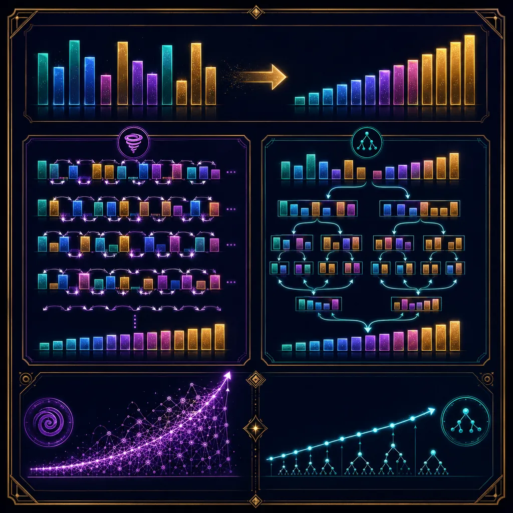
I’ll give you a sorting algorithm — assign it a complexity class. Simple algorithms are O(n²), clever “divide and conquer” ones are O(n·log n).
What just happened?
Sorting — arranging data in ascending or descending order — is one of the most common operations in computer science, and performance is decided by the choice of algorithm. We raised the number of elements to 1,000 and compared two strategies: simple bubble sort and clever merge sort.
Computational complexity (big-O notation)
Complexity describes how the number of operations grows with the data size . Simple algorithms (bubble sort, selection sort) compare every element with every other, so they perform on the order of:
Clever algorithms — merge sort (devised by John von Neumann in 1945) or quicksort — thanks to the “divide and conquer” strategy (split the data into halves, sort recursively, merge the sorted parts) achieve:
Why such an enormous difference?
For small n the difference is tiny. But for n = 1000 that is ~1,000,000 operations () versus ~10,000 () — a hundred times fewer. Sorting a million elements with an algorithm takes trillions of operations (hours, even days), while — a few tens of millions (a fraction of a second). The choice of algorithm decides whether a program runs for seconds or years.
A foundation of theoretical computer science
Complexity analysis lets us predict whether a program can realistically be run, even before we write it. That is why standard libraries (in Python, Java, C++) use algorithms of order internally, rather than naive quadratic loops.
Why this matters for your exams:
The topic of complexity itself lies outside the high-school curriculum (it straddles mathematics and computer science), but logarithms and the growth rate of functions certainly are on it. Being able to compare how grows faster than is the same intuition you need in problems about functions and sequences.
Remember: the number of operations grows with n according to the algorithm’s complexity — bubble sort , merge sort — and the difference escalates sharply with the data size. That is why the choice of algorithm, not a faster computer, decides what can be computed.
Theory & formulas
Time complexity
The number of operations as a function of the data size is described by big-O notation:
- bubble sort:
- merge sort:
Why such an enormous difference
For : , while — about a hundred times fewer operations.
Divide and conquer
Merge sort splits the data in half, sorts the parts and merges the results — hence the factor (the number of levels of division).
Notation: the number of elements, the order of the number of operations, logarithm.
Frequently asked questions
›In what time does an efficient algorithm sort?
In time of order n·log n (e.g. merge sort), much faster than n² (bubble sort).
›What is computational complexity?
A description of how the number of operations grows with the data size n (big-O notation).
›Who devised merge sort?
John von Neumann, in 1945 — a “divide and conquer” algorithm with complexity O(n·log n).
Teaching? Embed this experiment on your site.
Free widget — paste it on your school site, blog or notes. It links to the full version.